Matlab的学习
关于Matlab的学习,持续更新
前言
本学期的两门课,图像处理和数据挖掘可能或多或少涉及Matlab的使用,还是未雨绸缪一下吧。
安装
天津大学没有Matlab正版权限,那只能含泪使用盗版了。。。
迅雷网盘链接
但愿天下资源无人发度盘
找迅雷的资源是因为手里有破解版迅雷(小红车应用程序分类里搜到的破解版。。。)
具体安装流程 MATLAB2024 B下载安装教程
我进来力!
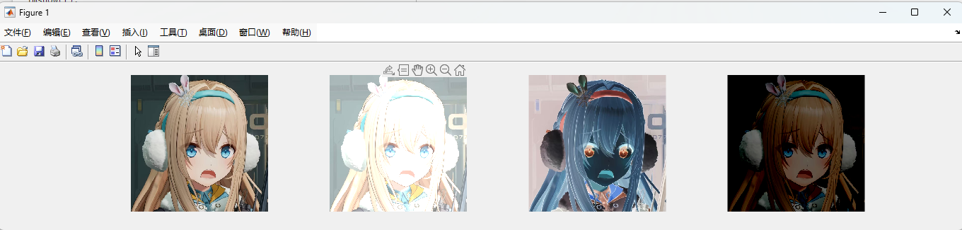
图像大小以及旋转操作
1 | clc;clear; |
分别是原图,大1.5,小1.5,旋转保留原分辨率,旋转保留图像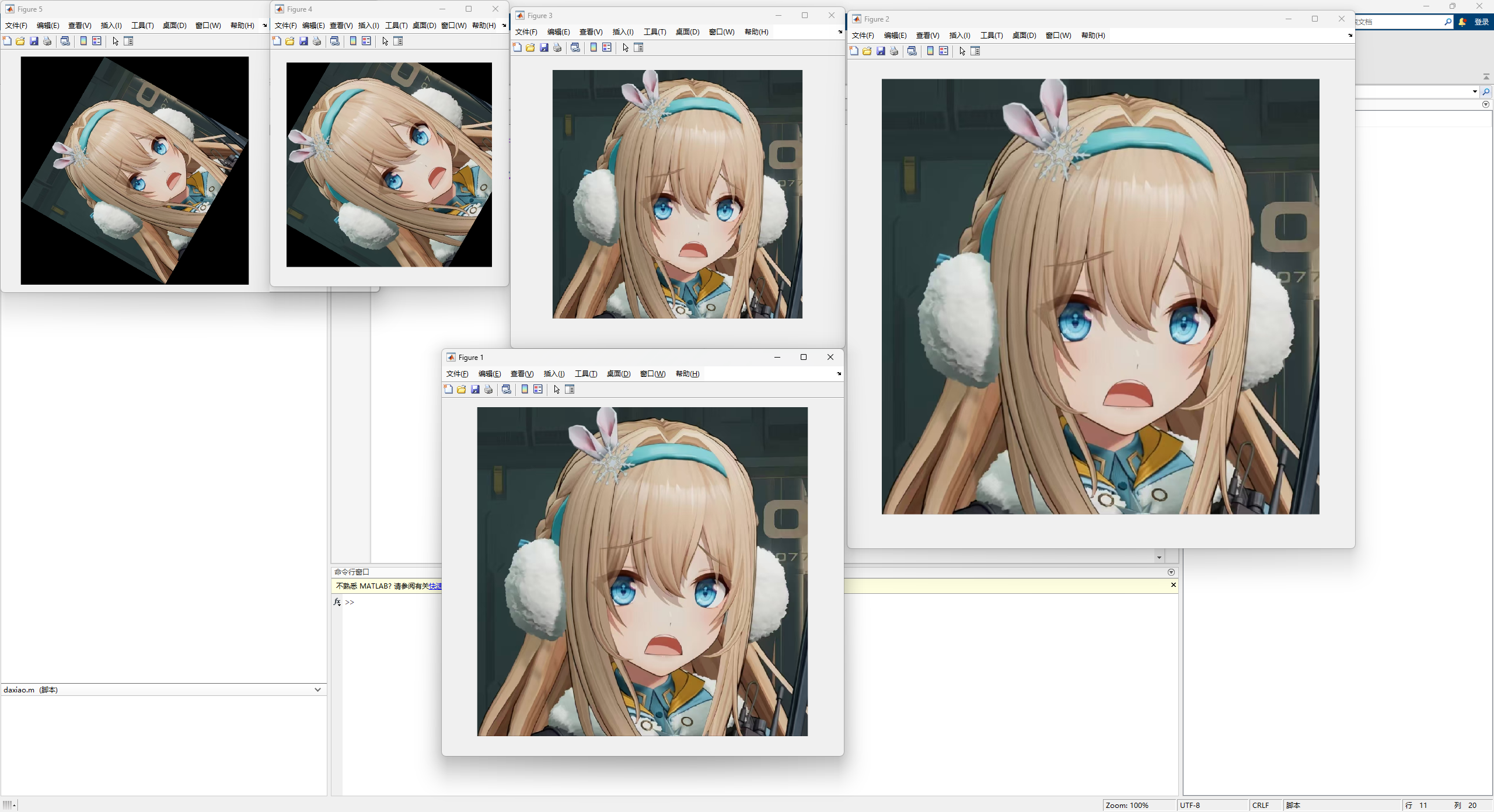
图像读写
1 | clc;clear; |
能做到图片类型的转换,有点意思
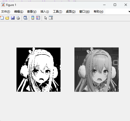
图像灰度,黑白等操作
二值与灰度
1 | clc;clear; |
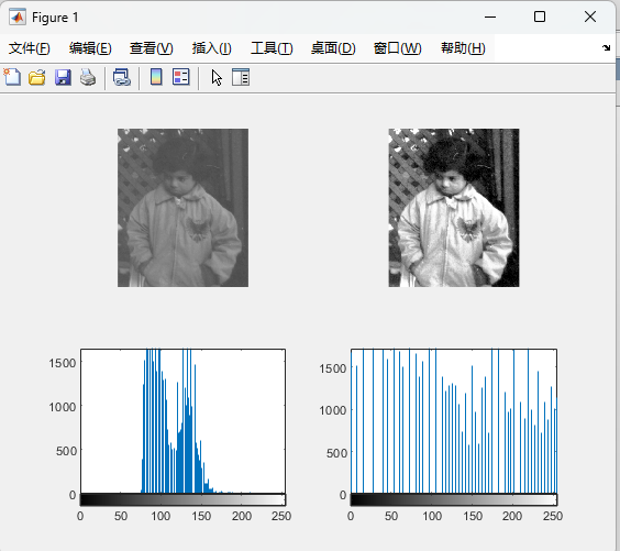
直方图与均衡化
1 | clc;clear; |
灰度变换
主要是imadjust的使用,第一个括号为原来的灰度范围,第二个为目标的范围
此外adjust还有不少玩法,https://blog.csdn.net/Ibelievesunshine/article/details/79958899
1 | clc;clear; |
噪声消除
RGB图像的噪声消除可能要放在后面再说了
以下都是灰度图像的噪声消除,话说这个不叫噪点吗。。。?
均值滤波
原理是将周围一定范围的像素点的值取平均,从而将噪声的影响减小
1 | clc;clear; |
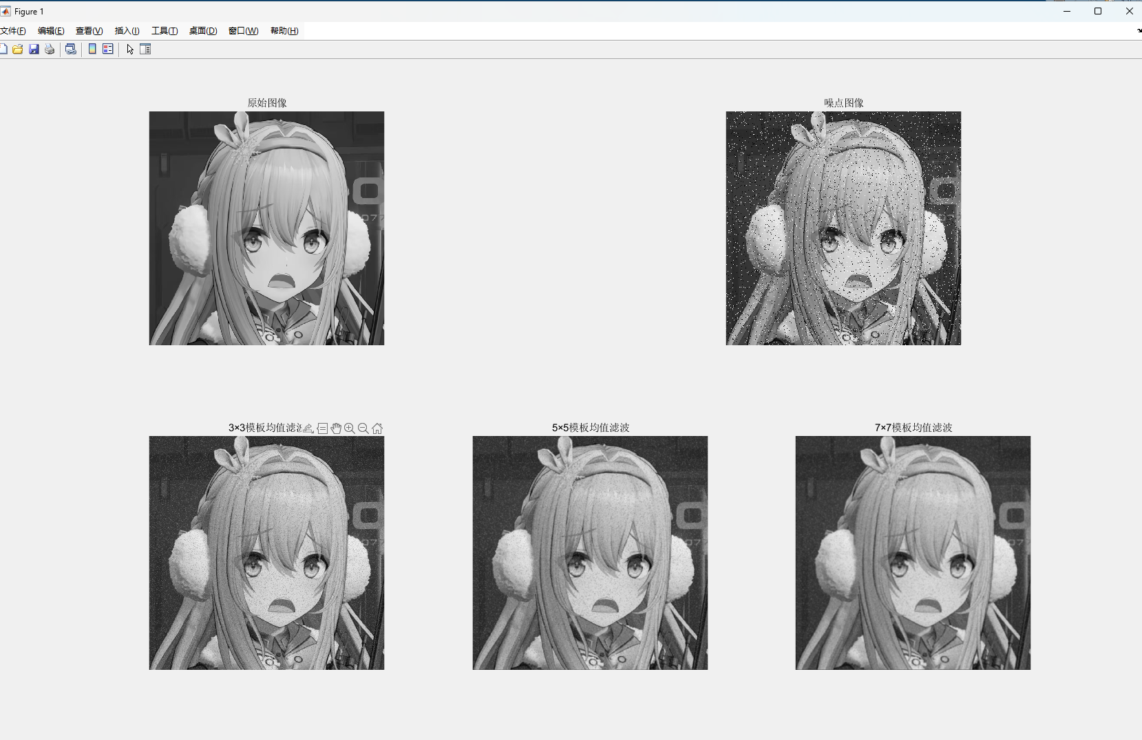
中值滤波
同理,取的是中值
1 | clc;clear; |
边缘检测
w4 w8这种是对应类型的滤波器,心里清楚即可
g4,g8是滤出来的, G4,G8是原图 减 滤出来的
感觉这个东西能玩那种模拟恐怖描边图的
1 | clc;clear; |
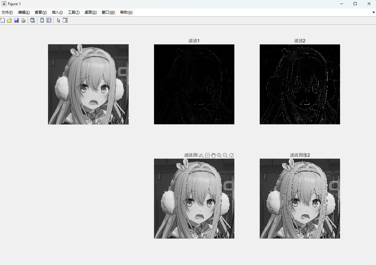
这个滤波2效果不错,来个颜色替换就能成了。
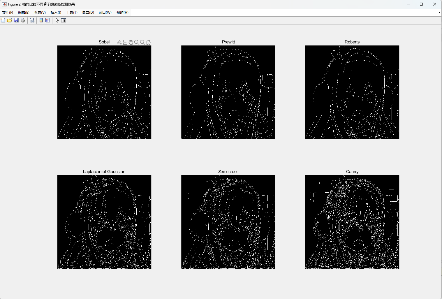
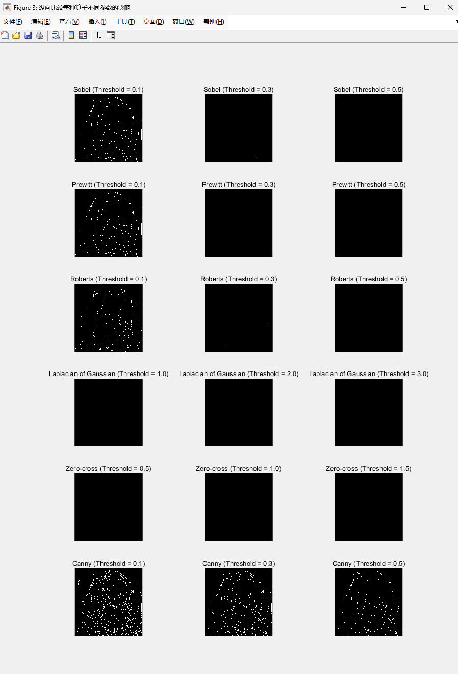
常见的边缘检测
六种常见的边缘检测方式以及填入不同参数的效果,具体原理搞不懂。。。
1 | clc;clear; |
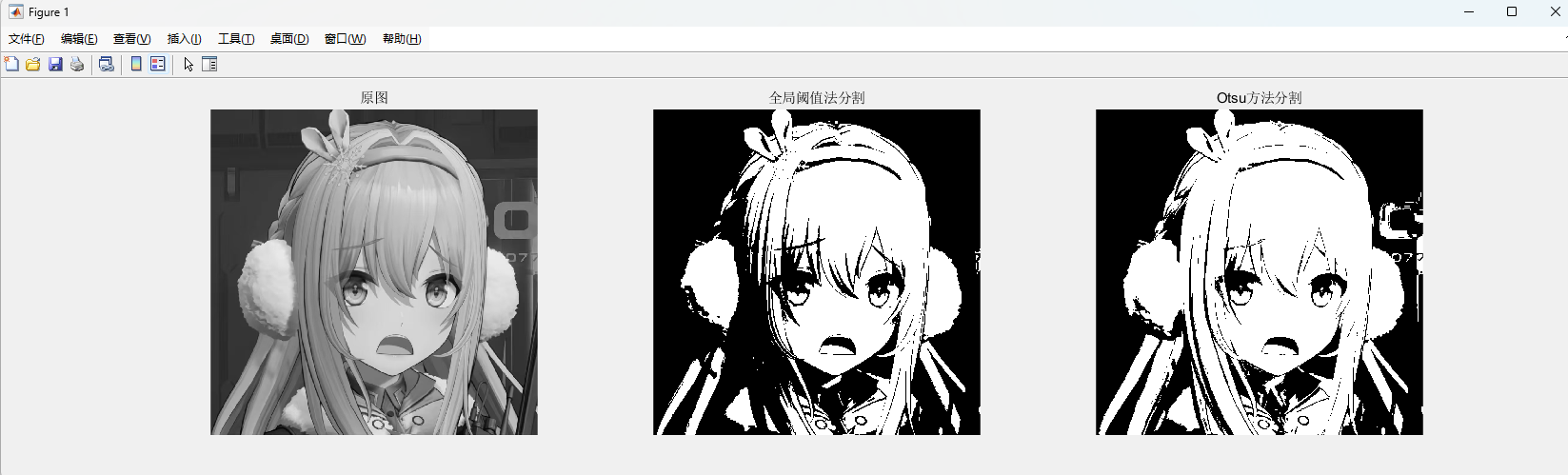
图像分割
在这里先学习两种方法:
全局阈值法,即手动选择区间,然后非黑即白;
Otsu方法,通过graythresh函数找到这个合适的阈值(全自动的?)
1 | clc;clear; |
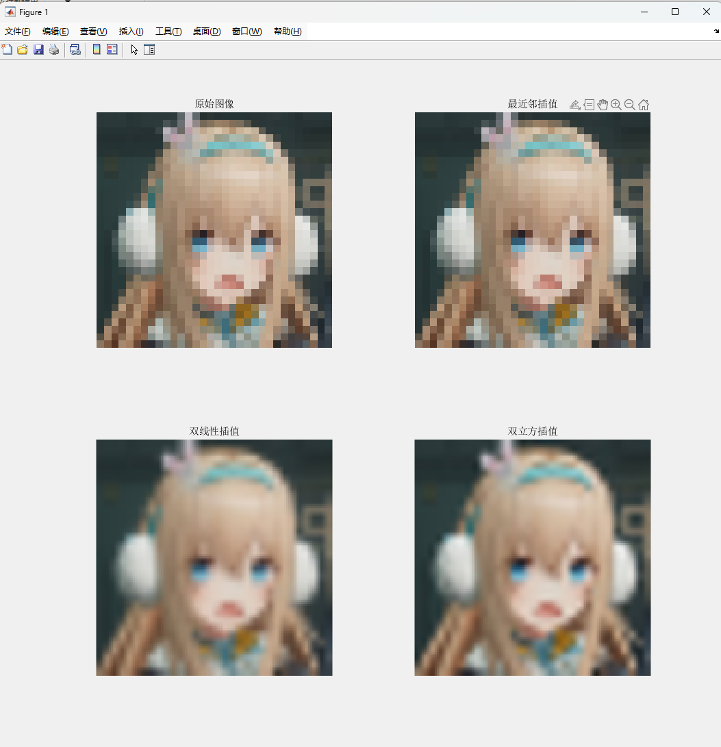
图像缩放
最近邻插值法:使用距离目标像素最近的源像素的颜色来填充目标像素的颜色值。
双线性插值法:使用目标像素周围的四个最近的源像素来计算目标像素的颜色值。
双立方插值法:使用目标像素周围的16个最近的源像素来计算目标像素的颜色值。
效率从高到低,图像质量从低到高。 (也许就是抗锯齿???)
1 | clc;clear; |
一个32*32的icon图片的放大。可以看出双立方插值将图像放大后效果最好
一些有趣的理解方式(这下看懂了):
| 抗锯齿技术 | 对应插值思想 | 性能消耗 | 质量 |
|---|---|---|---|
| SSAA | 双立方插值 | 非常高 | 极佳 |
| MSAA | 双线性插值 | 中等 | 很好 |
| FXAA | 智能滤波 | 很低 | 一般 |
| TAA | 多帧融合 | 低 | 很好 |